Digital Galton Board

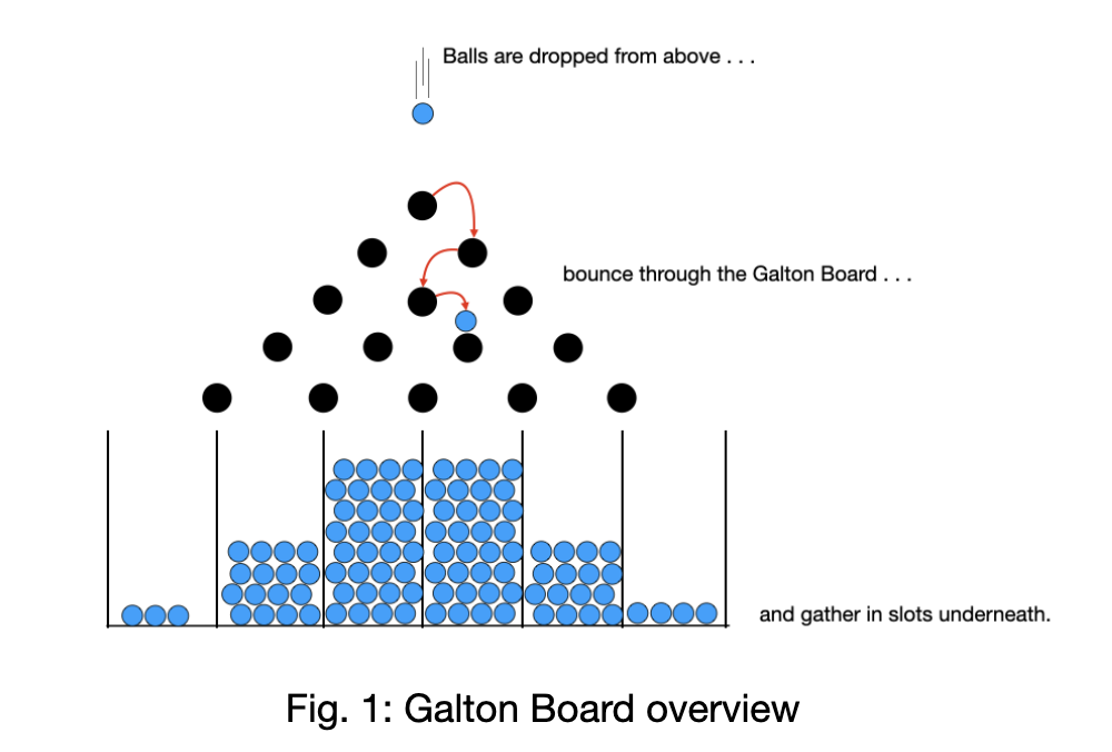
We designed and built a digital Galton board, a traditional game involving a ball or balls sent through a series of rows of pegs. This project involved a number of challenges, such as modelling real-world collision physics, VGA graphics display using VGA, and sound generation. Synthesizing the diverse aspects of the project in code and hardware was a key component of this project, especially timing optimization. Our system animates hundreds to thousands of balls at ~30 frames per second using fixed-point arithmetic for real-time physics, a VGA pipeline for display, and DMA triggered audio to produce a brief “thunk” sound on peg impacts without interrupts overhead. Hardware was added to provide additional features and adjust parameters. A potentiometer provides a simple, low-latency interface to tune parameters, in this case ball count and coefficient of restitution. We also overclock the microcontroller and apply optimization throughout, to increase the number of balls which can be modeled simultaneously without sacrificing the frames per second. Furthermore, we plot a live histogram which converges towards the Gaussian predicted by the CLT (Central Limit Theorem) as rows and trials increase. In this Lab report, we will discuss our hardware model, histogram generation, physics behind our implementation, optimization and results.

Our program consists of a main function to be run at boot and two protothreads, for simulation updates and VGA animation, respectively. In the main part of the program, we brought the system from the initial circuit to a stable, interactive demo of the Galton Board. We configured the higher system clock to sustain ~30fps, initialized the PIO-driven VGA pipeline to provide a 640x480 screen, and connected the user physical controls using the potentiometer and denouncing the push button to switch modes between ball count and bounciness. We also integrated a precomputed “thunk” sound,which will be output by a speaker when the ball hits the peg. DMA channels were used to send this to the DAC and speaker over SPI, so the audio feedback wouldn’t interfere with rendering or causing overclocking.

The runtime was split into two threads. One is for animation, which draws and erases the balls, pegs, text, and histogram. It renders the 16 rows of pegs and updates fixed-point physics. Additionally, we aligned a right-side histogram of 17 bins (0–16) to match the 16-row board’s chutes, and count each ball exactly once below a finish line near the bottom, scaling bar heights to the current maximum.We verified the behavior of our protothreads by checking the raspberry Pi’s onboard LED light to see if it passes timing. If not, it will flag the missed deadlines during tests. We also needed to verify the VGA and potentiometer was functional.

For validation, we first confirmed that VGA sync remained stable under load. The on-board LED correctly flagged frame deadline misses during stress tests, including maximums of 3000, 4000, or even 100000 balls. The potentiometer produced smooth, real-time adjustments in both modes, and mode-cycling was reliable after debouncing. Finally, the collision “thunk” triggered cleanly without jitter or lag, even with many balls on screen.

A key component was accurately modelling collision physics. For purposes of simplicity, we only modeled collisions between balls and pegs, not between balls, ie. collisions between a moving and stationary object.

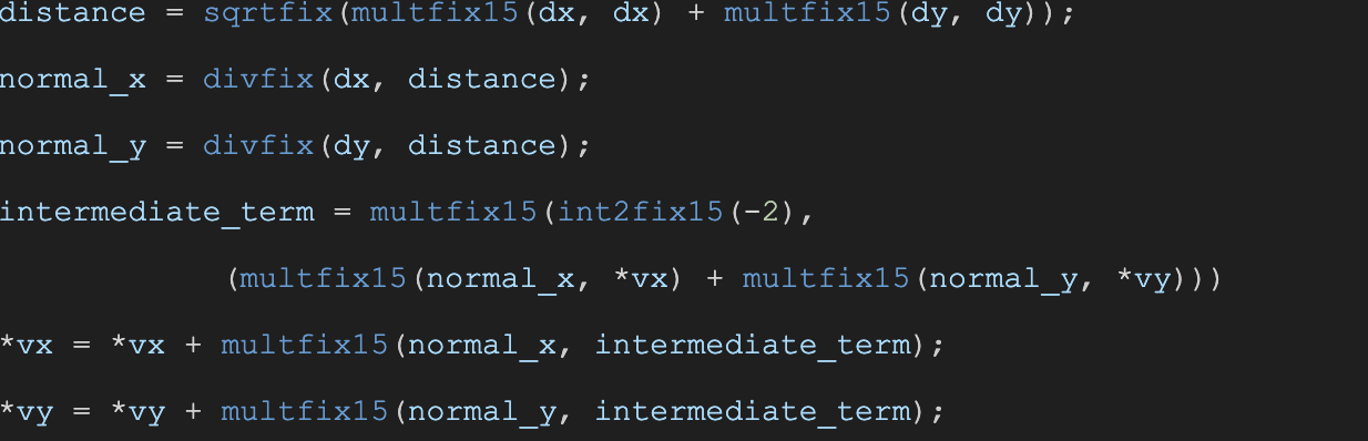
We used the equation for change in velocity derived in the “The physics of colliding balls, with coefficient of restitution” webpage (figure X), where mass M of the peg is infinite and the vectors rm and rM represent the positions of the centers of mass of the peg and ball in question.

In the code, we created a variable “distance” representing the difference in positions between the peg and the ball, as well as variables “normal_x” and “normal_y” representing the portions of this distance in the x and y directions. These are then used to calculate the change in velocity for the x and y directions.

Additional actions are performed to account for issues arising in the simulation which differ from real-world physics. For instance, since updates to the simulation occur at a granular time scale, instead of continuously as in real physics, sometimes the ball would move inside the perimeter of a peg. As a result, we needed to include code which “teleports” the ball back outside of the peg upon update. Additionally, we had to add a line of code to apply gravity to the y velocity on each cycle.

Further, we decreased velocity by multiplying by a “bounciness” coefficient to simulate the coefficient of restitution. This takes into account energy lost to sound, vibration, and heat in collisions which are not perfectly elastic.

In an ideal case, a Galton Board will result in a Gaussian distribution. This relies on the assumption that all ball bounces’ directions (left or right) are completely independent of all previous bounce results, and identically distributed between each side of the peg (a 50% chance of bouncing left or right). However, in our simulation, we attempted to model a nonideal, real-world Galton Board. In this model, the direction each ball hits the peg is dependent on how it hit and bounced off the previous peg, both removing independence and identical Bernoulli distribution. However, as a large number of balls are dropped, due the CLT generalization for mixing processes, the board approaches a Gaussian anyways, since as a ball continues to bounce, earlier rows’ bounces become less important. As a result, Galton Boards with more rows better approximate a Gaussian distribution.

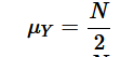
Our model, with sixteen rows and seventeen bins, had an ideal mean of eight (the middle bin in the seventeen-bin histogram), and a standard deviation of 2.06.

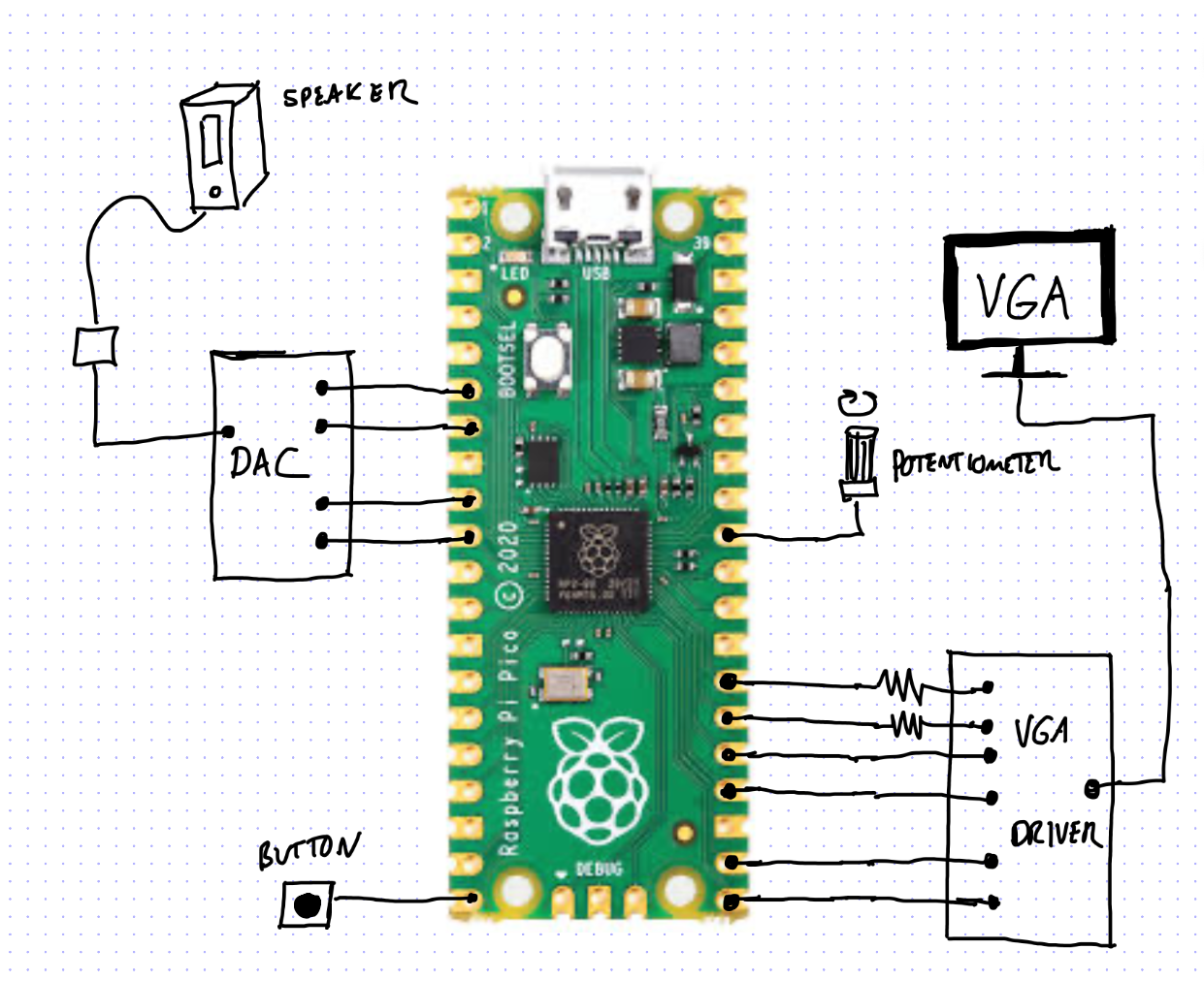
Users interact with an external button and a potentiometer to adjust the parameters of the Galton board (refer to the hardware diagram below for the setup). Upon boot, the program initializes in "mode 0," where the maximum number of balls that can be animated at 30 frames per second are dropped and the “bounciness” coefficient is set to a default value of 0.5. In "mode 0," adjusting the potentiometer does not affect any parameters, including the number of balls dropped or their bounciness.

When the user presses the external button once, the program transitions to "mode 1." In this mode, adjusting the potentiometer changes the number of balls dropped. Pressing the button a second time switches the program to "mode 2," where turning the potentiometer modifies the bounciness of the balls. Pressing the button once more returns the program to "mode 0." Repeated button presses cycle through all modes: 0, 1, and 2.

In the program main, the external button is connected to GPIO 15. It is set as a GPIO input, with the internal pull-up resistor on.

In the global scope, we declared an integer variable “mode” and initialized it to 0 to indicate that the program is booting into “mode 0.”

Inside the while loop of the parameter update thread (originally the user serial input thread in the original animation.c demo code), we first evaluate which mode we are currently in. These conditional statements determine how the potentiometer input is interpreted. In mode 0, the potentiometer input is ignored.

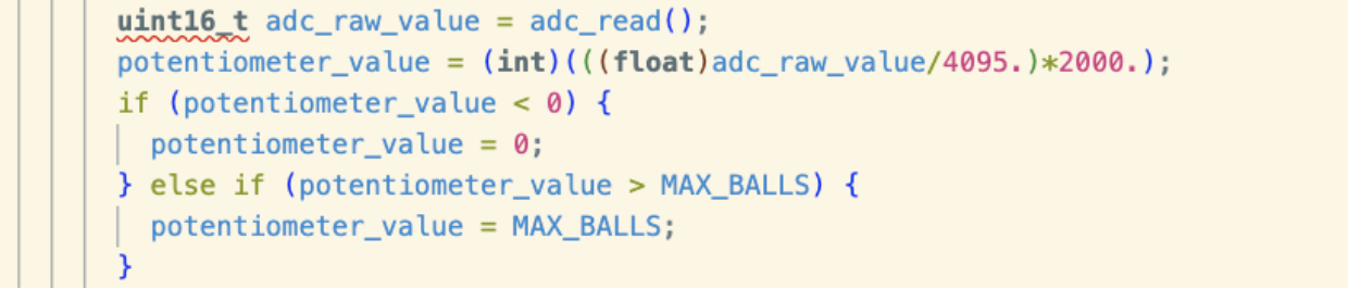
In mode 1, we scale the raw ADC reading from the potentiometer to control the number of balls dropped in the animation. On the RP2040, as with most microcontrollers, the ADC is a 12-bit converter, producing raw digital values between 0 and 4095 (212 - 1). The raw ADC value returned by adc_read() is first converted to a floating-point number and divided by 4095.0 to normalize it to a range of 0.0 to 1.0, representing the input voltage fraction. This normalized value is then multiplied by the maximum number of balls (2000 in the image below) and truncated to an integer, giving a final value between 0 and 2000 that specifies how many balls should be dropped.

In mode 2, the same ADC reading from the potentiometer input is used, but this time it controls the bounciness parameter in the collision physics. The raw ADC value is first normalized by dividing by 4095, producing a floating-point value between 0.0 and 1.0. This normalized value is then multiplied by the maximum bounciness (set to 1.0) and converted to a fix15 fixed-point format (with 16 integer bits and 15 fractional bits). The resulting fixed-point value, ranging from 0 to 1 with 15-bit fractional resolution, determines how elastic the ball collisions are in the simulation.

When displaying the bounciness value on the VGA screen, the 15-bit fractional precision is truncated to show only two decimal places for readability.

Button press detection occurs within the same thread. Multiple button presses may be caused by the bouncing of pressing a physical button, creating a short period of unstable inputs (rapid switching from high voltage to low voltage) to the GPIO. A hardware solution to this issue involves adding a resistor and a capacitor to create a low-pass filter that smooths the signal. However, we chose to implement a software solution by employing a finite state machine debouncing algorithm, which introduces a buffer cycle to stabilize the button input. We added the debouncer state machine we implemented in Lab 1, the bird song synthesizing lab, and made some modifications to better suit our needs.

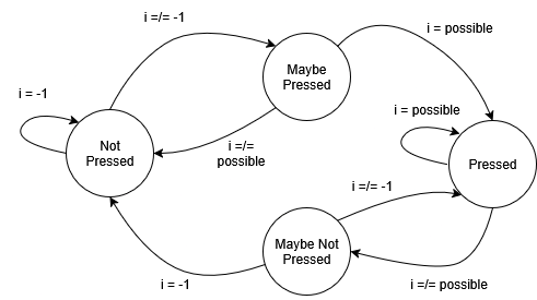
After the button press stabilizes, we increase the global counter, button_press_count, by 1. The program then checks the counter to decide which mode to activate. On the first button press, mode is set to 1. On the second button press, the mode is set to 2. On the third button press, mode is returned to mode 0. Each button press advances the program to the next mode in sequence, cycling through modes 0, 1, and 2.

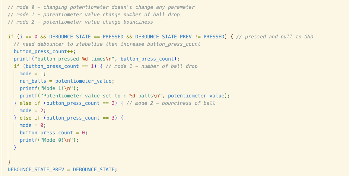
After cycling through all three modes, the button_press_count counter resets to zero so that subsequent presses continue the sequence.

Finally, the current debounce state is stored in a variable called DEBOUNCE_STATE_PREV to ensure accurate detection of the next button transition.

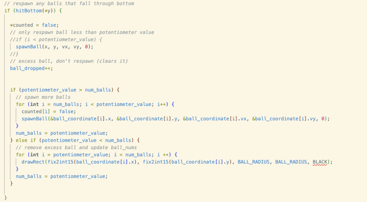
When the program operates in mode 1, twisting the potentiometer adjusts the number of balls actively dropping in the animation. The ADC reading from the potentiometer is scaled and stored in the variable “potentiometer_value,” which represents the desired number of balls to be dropped. The program continually compares this value with “num_balls,” which tracks the number of balls currently being animated and scheduled for respawn.

If the user turns the potentiometer to increase the number of balls, the program dynamically spawns additional balls until the current count matches the potentiometer setting. Conversely, if the potentiometer is turned to reduce the count, the program stops respawning the excess balls once they fall off the screen.

The logic governing the spawning and removal of the balls can be summarized in the following pseudocode:

                        
                            num_balls = number of balls to be spawned/go through collision physics

                            Potentiometer_value = desired drop ball value

                            Current_num_balls = actual number of balls already animated/respawned

                            If potentiometer_value > num_balls:

                                    Spawn more balls

                                    Update num_balls

                            If potentiometer_value < num_balls:

                                    Remove extra balls by not respawning them        

                            Extra or excess balls = (current_num_balls > potentiometer value)

                        
                    

To implement this behavior, we first structured the program so that each ball instance is processed in the ballCollidePeg() function, which takes the ball’s position, velocity, and index in the ball_coordinate array as parameters.

At the global scope, a Boolean array is declared to track whether each ball has already been counted in the histogram after reaching the bottom of the screen. The index i of each ball corresponds directly to the index in the counted array (ball_coordinate array and counted array both of length MAX_BALLS), which also determines whether that ball is eligible for respawn.

At the end of the collision update, ballCollidePeg() calls wallsAndEdges(), passing in the ball’s identifier, index i in the ball_coordinate array. The wallsAndEdges() function handles left and right wall collision detection, updating ball positions and velocity after hitting a left or right wall (bounded by screen width), and determines whether to respawn any balls that fall through the bottom of the screen.

Within wallsAndEdges(), when a ball reaches the bottom of the screen (hitBottom(*y) returns true), the program resets the ball’s counted[i] flag and determines whether the ball should be respawned.

If the ball’s index i is less than the potentiometer value, it is respawned by calling spawnBall(), ensuring that only the desired number of balls remain in the animation. When the potentiometer_value exceeds num_balls, new balls are spawned in a loop from num_balls up to potentiometer_value, dynamically increasing the total number of animated balls. Conversely, if the potentiometer_value is less than num_balls, the excess balls are erased from the screen using drawRect() with color set to BLACK, and are not respawned. Each ball instance checks its index i relative to the current loop iteration to determine whether it should respawn. Finally, num_balls is adjusted to reflect the current number of balls to be animated and respawned in the animation.

The histogram was generated by converting each ball’s final horizontal position into a discrete bin and then incrementing that bin’s count to be exactly 1. When a ball crosses a fixed line near the bottom of the display, I map its x-coordinate to a bin index by subtracting the leftmost bar’s x origin (HIST_START_X) and then dividing it by the constant chute spacing (HORIZONTAL_SPACING). This yields an integer index from 0–16 which gives 17 bins for a 16-row array (values outside 0–16 are ignored). To avoid double counting in the later frames, we set counted[i] = true right after incrementing the bin (and reset it on respawn). Drawing happens each frame in drawHist(): for each bin i, I compute a proportional height h = (int)((float)50 * fix2float15(hist_data[i]) / fix2float15(hist_highest)); and paint a bar using the fillRect function, then clear the space above the bar to prevent ghosting. The histogram is rendered every frame by scaling each of the bin’s counts to a fixed pixel height using the largest observed bin as a reference. This helps keep the chart more readable and stable as more balls come into the frame. The count of the ball is maintained in integer form for stats and also stored as a fixed-point (fix15) copy for the drawing routine, which matches the lab’s real-time VGA constraints.

Our VGA screen displays:

• Current mode of the program
• Current number of balls being animated
• Total number of balls that have fallen through the board since boot
• Bounciness of the balls
• Time since boot

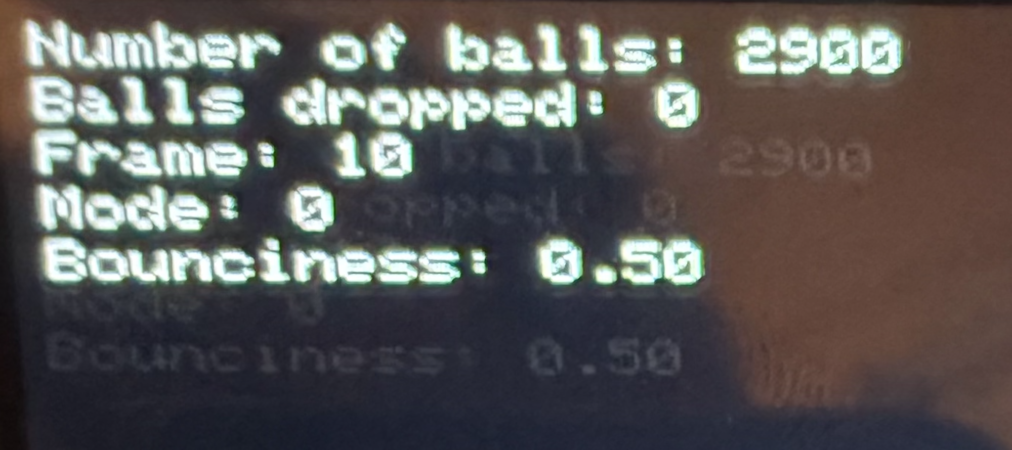
These values update continuously within the animation loop on core 0, ensuring that the display reflects the most recent simulation state. Later, when optimizing the code, some values are updated and displayed less frequently if the values are updated less frequently.

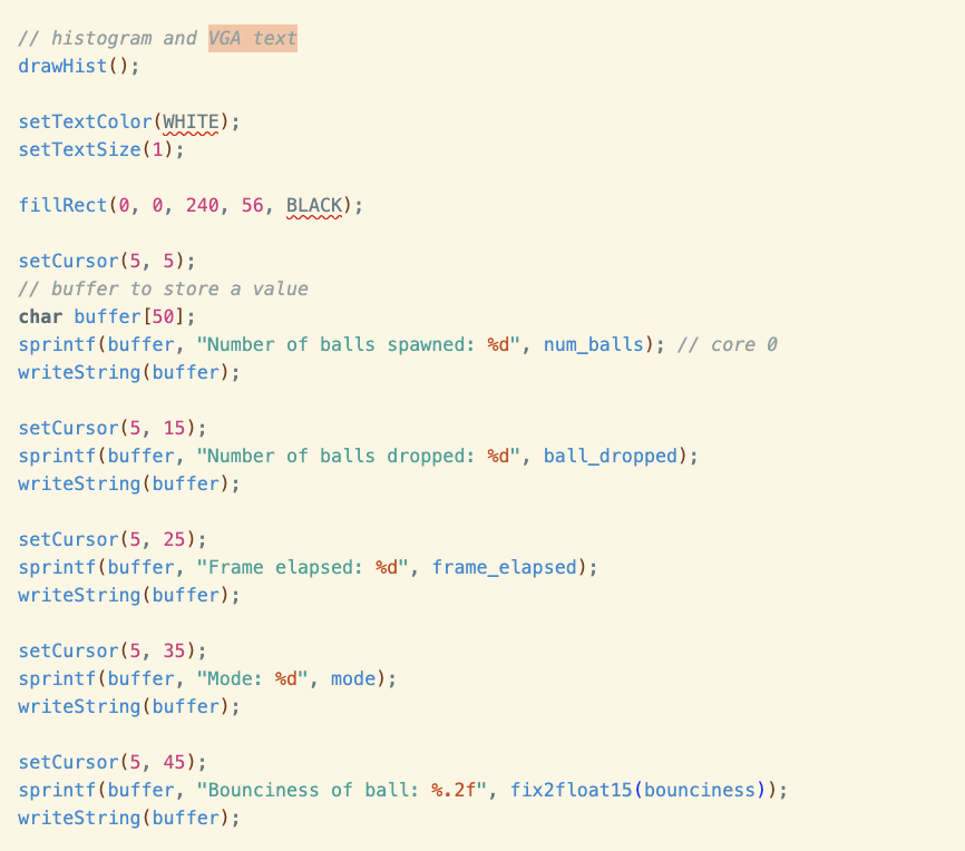
Before each frame update, a black rectangle is drawn over the text area using fillRect() to clear any previous text, preventing overlap from prior frame updates. The setCursor() function from the vga16_graphics_v2 driver positions where the text will display on the screen. writeString() draws the text to the screen.

To measure the elapsed time since boot, the function time_us_32() is called at the beginning of each animation loop iteration. This function returns the number of microseconds since the program started running the RP2040, allowing us to monitor frame timing. Begin_time stores this timestamp, and the frame_elapsed variable counts the number of frames that have been drawn since startup, tracking total animation duration.

Each time a ball hits a peg, a “thunk” sound must be generated. To this end, the RP2040 is wired to a digital-to-analog converter (DAC), which sends an output signal to a speaker. The RP2040 communicates with the DAC using Serial Peripheral Interface (SPI) channels. In SPI communication, data is shifted from the “main” device into a “secondary” device, and vice versa.

Since the collision math as well as the VGA display require as much time as possible in the CPU, Direct Memory Access (DMA) channels were used to directly transfer data from memory to the SPI data register port. For this project, we used two DMA channels, for control and data respectively. The control channel is used to fetch the sound data, and is chained to the data channel, which sends the data to SPI. The DMA channel mask function is called during the animation protothread; no calculations are made, and the data is sent to the SPI port without significantly impacting timing.

To make the “thunk” sound, we created a table of data to model a sine wave, to be progressively sent to the DAC. Additionally, we did not ramp the sine wave, since the popping sound artifact, which usually must be removed for smooth sound generation, is in this case desirable, as it sounds remarkably like a thunking noise.

Our system runs on the RP2040 and drives a 640x480 VGA display while sampling a potentiometer, reading a push-button, blinking the on-board LED, and outputting a short “thunk” sound via an DAC using DMA and SPI communication. We clock the MCU to 250 MHz to maintain ~30 fps with many balls in flight.

VGA output uses the lab’s PIO-driven pipeline and a simple resistor DAC. The pins follow the template in our code header: GPIO16, GPIO17, GPIO18/19, GPIO20, and GPIO21, with VGA ground tied to RP2040 GND. PIO state machines handle HS/VS and pixel timing while DMA streams pixel data, so the CPU can focus on physics and displaying each frame. The button does not control the state machines physically but instead it cycles modes in software, where mode 0 is the baseline, mode 1 potentiometer adjusts ball count, and mode 2 potentiometer adjusts bounciness. The on board LED serves as a frame deadline indicator in case it doesn’t support the 30 fps anymore.

Audio for the “thunk” is precomputed into a 256-sample table and sent to an SPI DAC using a two-channel DMA setup to avoid interrupts. We use SPI0 on GPIO5, GPIO6, and GPIO7; GPIO4 is configured by SPI but unused by the DAC. A timer-paced throttles the data DMA so playback occurs at a fixed rate, and a small control DMA transfers arms each burst. On each validated peg collision, we trigger the control channel to play a single thunk cleanly without impacting frame timing.

The potentiometer provides real-time control without interrupts. It is wired to ADC0 on GPIO26, and we initialize it with adc_init(), adc_gpio_init(26), and adc_select_input(0). In the UI thread we read the 12-bit value from adc_read() (range 0–4095) and map it directly to our parameters depending on the current mode: in Mode 1 the reading sets the ball count (potentiometer_value clamped to [0………MAX_BALLS]), and in Mode 2 it sets the bounciness by converting to Q15 (bounciness = float2fix15(adc_raw/4095.0f)). The update is applied immediately, so turning the knob changes the number of active balls on the next frame.

The goal of is to animate as many balls as we can while meeting the 30 frames per second timing deadline. In mode 1, twisting the potentiometer adjusts the number of balls dropped. If the 30fps deadline is missed, the Raspberry Pi Pico on-board LED turns on.

The graph below summarizes the maximum number of balls we can animate while meeting the deadline under various optimization scenarios.

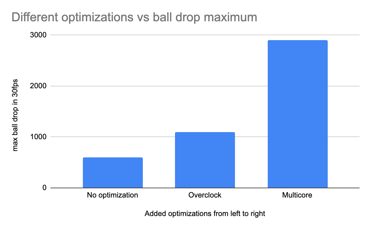
1. No optimization - 600 balls
Without applying any of the optimizations discussed in the lecture, we can animate a maximum of about 600 balls while still meeting the deadline.

2. Overclocking - 1100 balls
We overclocked our system clock from 125MHz to 250MHz. In the animation.c file, we updated the argument passed to the csdk set_system_clock_khz() function from 150000 to 250000. The program now runs at 250 million clock cycles per second.

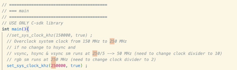
The hsync and vsync PIO state machines execute instructions at 25 MHz. Our VGA screen demands that we send a new value to the RGB pins at precisely 25 MHz. To maintain this 25 MHz pixel clock time (same as PIO instruction time, since each PIO instruction takes a single cycle), we can set the clock divider to 5.

250 MHz / 5 = 25 MHz

However, when we actually set the clock divider in our hsync and sync pio state machines to 5, our right side of our Galton Board seemed to go past the right edge of the VGA screen. So instead, we set the clock division to 6, to get 250 MHz /6 = 20 MHz.

The rgb PIO state machines execute instructions at the full 125 MHz system clock rate. To accommodate the change of system clock rate to 250 MHz, we set the clock divider in rgb.pio to 2.

250 MHz/2 = 120 MHz

This doubling in system clock rate allows us to animate almost double the number of balls.

3. Multicore - 2900 balls
We made a second version of the animation thread and put it on core 1. Both core 0 and core 1 work on the animation simultaneously. Because we didn’t implement any ball-to-ball collisions, this implementation of parallelization is quite straightforward. A mutex was used to lock resources shared by the two cores.

By having both core 1 and core 0 animate balls, we were able to animate almost more than triple the previous amount of balls.

4. Alpha Max Beta Min - ___ balls
Next, we checked our entire program to ensure that there is no expensive floating-point arithmetic. In our ball collision logic, we originally computed distance by converting the fixed-point argument dx*dx + dy*dy to a floating-point value, computing the square root of the floating-point value, then converting the floating-point value back to fixed-point to be used in further calculations.

We were able to avoid doing floating-point square roots by computing the root sum of squares using the alpha max beta min algorithm. We let alpha equal 1/1 and beta equal 1/4, for the largest error to be 11.61%.

When we test our program, we realized that we ran out of memory. Our program can’t compile if we increase MAX_BALL to 2900 to 3000, before the LED turns on. To get back more memory, we can changed the pio state machines and vga driver to run 1-bit resolution (1 color) instead of 4 bit resolution (16 colors), but we decided to get checkoff here (while trying to get back more memory and failed in the time we had).

Below are some other optimizations we would have made and test:

5. Bit shift instead of multiplying by -2 - ___ balls

6. Bounciness Calculation - ___ balls

7. 2x2 pixel square ball - ___ balls

8. Guess which peg in collide row - ___ balls

9. Draw peg, pixel, update text only when necessary - ___ balls

10. Remove Print Statements - ___ balls
Print statements go through a UART channel, with a baud rate of 112500 and 10 bit times per character, making it very expensive. As a final optimization, we could have easily commented out print statements that were used for debugging purposes to get back more balls.

One issue we encountered in the lab is the VGA display crashing when we decrease the ball count with the potentiometers. Initially we thought it was because the ball was erased at the bottom of the frame and was never removed. However, since the issue only occurs when the potentiometer was turned lower, we tackled the logic behind it. One suggestion we got from Dr Adams was to make sure the potentiometer value never reached below 0. So we implemented a if statement that makes sure if the potentiometer is going into the negative direction, it will be hardcoded to 0. We also coded if the potentiometer value is less than the number of balls, then it will be erased from the board. This solved our crashing issue with the potentiometers.

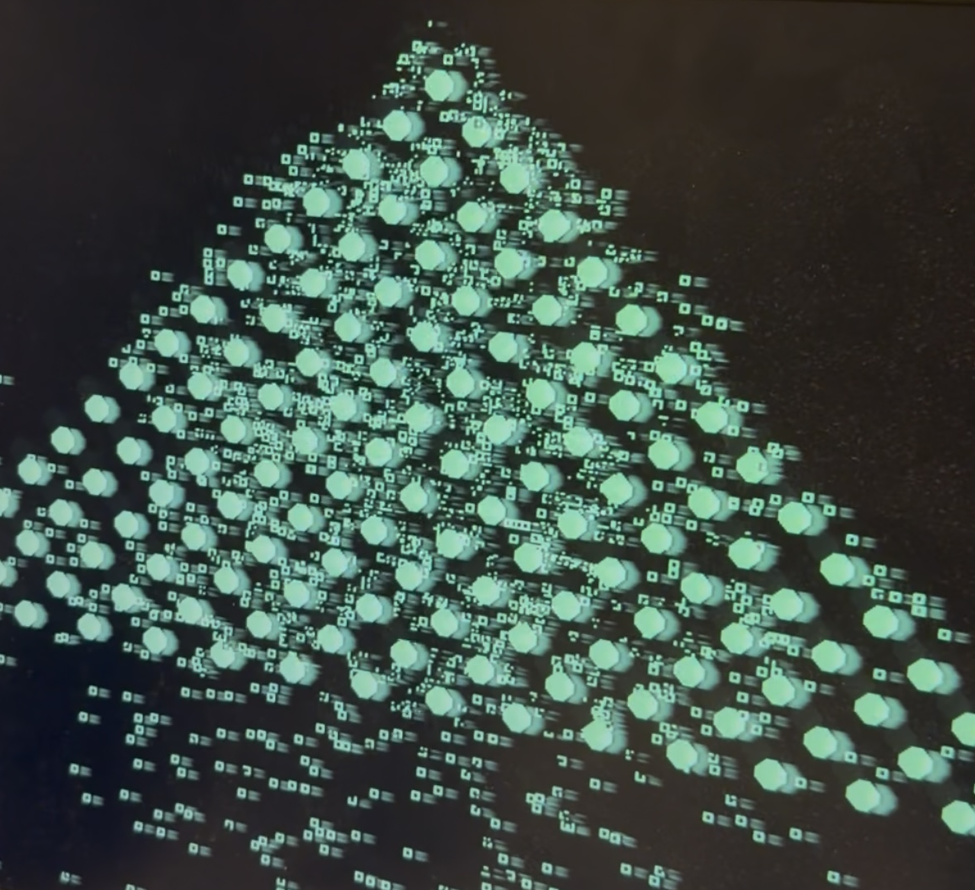
We also ran into trouble by introducing too many variables. Early on, we didn’t carefully review the provided parameters, so we defined our own and then edited both the lab’s parameters (boids) and our custom ones. That overlap created confusion about which variable controlled what and ultimately cost us the first week’s checkoff. We resolved it by restarting from a clean baseline, reading the provided interfaces carefully, and standardizing on the given parameters before adding any new ones. Another issue we faced was the ball always missing the first peg. This was a fairly simple fix: we position the peg closer to the ball drop point.

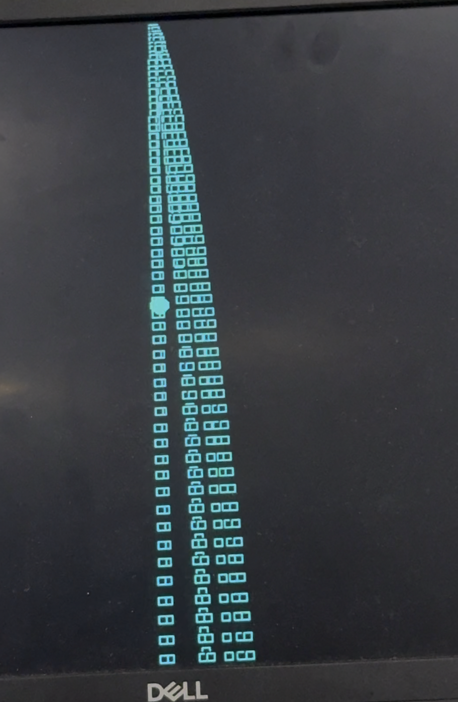
After unsuccessful attempts to erase and straighten the ball, we restarted from a clean baseline and replaced our extra BOID variable with the lab-provided definitions organized as C structs. This resolved state inconsistencies and made the code scalable. We initially brought up the system with a single hard-coded ball, then refactored to an indexed array of balls to support the larger populations needed in later weeks.

This lab exercise culminated in a successful Galton board and fruitful learning experience. All aspects of the lab, including ball generation, collision physics, VGA display, histogram, sound, and potentiometer meet or exceed expectations. Through strategic design and continual optimization, we were able to increase our throughput to almost 3000 balls onscreen at a time. Along this path, we ran into numerous challenges, but through thoughtful design and extensive debugging, our end result was a success. One thing we could have done differently is getting started earlier the first week, as we ended up missing a checkoff; this was rectified by starting work earlier for the second checkoff, and attending more lab sessions. Additionally, we could have performed more optimizations with more time, such as removing unnecessary VGA updates and print statements. Overall, this lab provided a solid foundation for continuing work in physics simulation, VGA, and external device communication using the Raspberry Pi.

Michelle Yang: Lead the writing and debugging of majority of the code/logic. Individually completed all optimizations.

Xia Yan Zhao: Individually wrote code for generating a histogram. Assisted immensely with debugging the program.